21. Multiple Integrals in Curvilinear Coordinates
d. Integrating in 2D Curvilinear Coordinates
6. Applications
We previously did Applications of Multiple Integrals in Rectangular Coordinates and we have done Applications of Double Integrals in Polar Coordinates. All of those applications can also be done using general two-dimensional curvilinear coordinates.
All the examples on this page of applications of double integrals in curvilinear coordinates will use the region between the paraboloids \(y=9-x^2\) and \(y=4-x^2\) in the first quadrant. Besides the two parabolas, the other \(2\) boundaries are the \(x\)-axis (\(y=0\)) and the \(y\)-axis (\(x=0\)). Find a curvilinear coordinate system for the region. Then find the Jacobian factor and the ranges of the coordinates to describe the solid.
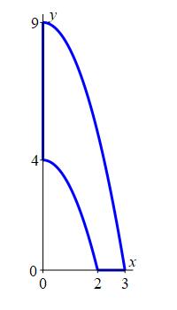
It seems obvious that we would like to to take one of the curvilinear coordinates to be \(u=y+x^2\) so that the \(2\) parabola edges are \(u=4\) and \(u=9\). But it is not obvious what to take for the other coordinate. For lack of a better choice, we take \(v=y-x^2\).
To compute the Jacobian, we need to solve for \(x\) and \(y\). To do this, we add and subtract the \(2\) equations: \[ u=y+x^2 \quad \text{and} \quad v=y-x^2 \] to get: \[ u+v=2y \quad \text{and} \quad u-v=2x^2 \] So our coordinate system is: \[ x=\dfrac{\sqrt{u-v} }{\sqrt{2}} \quad \text{and} \quad y=\dfrac{u+v}{2} \] From this, we can find the Jacobian factor: \[\begin{aligned} J&=\left|\begin{vmatrix} \dfrac{\partial x}{\partial u} & \dfrac{\partial y}{\partial u} \\[8pt] \dfrac{\partial x}{\partial v} & \dfrac{\partial y}{\partial v} \end{vmatrix}\right| =\left|\begin{vmatrix} \dfrac{1}{2\sqrt{2}\sqrt{u-v}} & \dfrac{1}{2} \\[8pt] \dfrac{-1}{2\sqrt{2}\sqrt{u-v}} & \dfrac{1}{2} \end{vmatrix}\right| \\ &=\left|\dfrac{1}{4\sqrt{2}\sqrt{u-v}}-\,\dfrac{-1}{4\sqrt{2}\sqrt{u-v}}\right| =\dfrac{1}{2\sqrt{2}\sqrt{u-v}} \end{aligned}\]
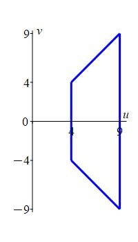
Two of the boundaries are \(u=4\) and \(u=9\).
The other \(2\) boundaries are:
The \(x\)-axis:
\[
y=0 \quad \text{or} \quad \dfrac{u+v}{2}=0
\quad \text{or} \quad v=-u
\]
The \(y\)-axis:
\[
x=0 \quad \text{or} \quad\dfrac{\sqrt{u-v}}{\sqrt{2} }=0
\quad \text{or} \quad v=u
\]
Here is a plot of the region in the \(uv\)-plane. This is a nice region
to integrate over. It is Type \(u\). So the \(u\) integral is on the outside.
Volume
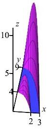
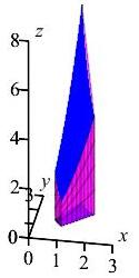
The volume under the a surface \(z=f(x,y)\) above a region \(R\) is: \[ V=\iint_R f(x,y)\,dA=\iint_R f(u,v)\,J\,du\,dv \]
Find the volume of the solid below the graph of \(f(x,y)=xy\) above region between the parabolas.
Area
The area of a region \(R\) is: \[ A=\iint_R 1\,dA=\iint_R J\,du\,dv \]
Find the area of the region between the parabolas.
Mass
The mass of a plate occupying a 2D region \(R\) with mass density \(\delta\) is: \[ M=\iint_R \delta(x,y)\,dA=\iint_R \delta(u,v)\,J\,du\,dv \]
Find the mass of the region between the parabolas if the mass density is \(\delta=x\).
Center of Mass
The center of mass of a plate occupying a region \(R\) with mass density \(\delta\) is: \[ \bar x=\dfrac{M_x}{M} \qquad \text{and} \qquad \bar y=\dfrac{M_y}{M} \] where \(M\) is the mass and the moments of the mass are: \[ M_x=\iint_R x\,\delta\,dA=\iint_R x\,\delta\,J\,du\,dv \] and \[ M_y=\iint_R y\,\delta\,dA=\iint_R y\,\delta\,J\,du\,d \]
Find the center of mass of the region between the parabolas if the mass density is \(\delta=x\).

Centroid
The centroid of a region \(R\) is: \[ \bar x=\dfrac{A_x}{A} \qquad \text{and} \qquad \bar y=\dfrac{A_y}{A} \] where \(A\) is the area and the moments of the area are: \[ A_x=\iint_R x\,dA=\iint_R x\,J\,du\,dv \] and \[ A_y=\iint_R y\,dA=\iint_R y\,J\,du\,d \]
Find the centroid of the region between the parabolas.


Average Value
The average value of a function \(f(x,y)\) on a region \(R\) is: \[ f_\text{ave}=\dfrac{1}{A}\iint_R f(x,y)\,dA =\dfrac{1}{A}\iint_R f(u,v)\,J\,du\,dv \] where \(A\) is the area.
Find the average value of the function \(f(x,y)=x^3\) on the region between the parabolas.
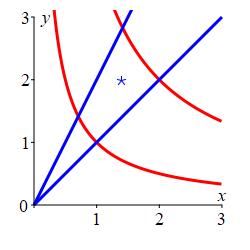
The exercises on the rest of this page refer to the diamond shaped region
discusssed in the last exercise on the
previous page. The boundaries are the curves \(y=\dfrac{1}{x}\)
and \(y=\dfrac{4}{x}\) in red and
\(y=x\) and \(y=2x\) in blue.
We already know:
The coordinates may be taken as \(u=xy\) and \(v=\dfrac{y}{x}\).
Then the boundaries are \(u=1\), \(u=4\), \(v=1\) and \(v=2\).
The coordinate system is \(x=\sqrt{\dfrac{u}{v}}\) and \(y=\sqrt{uv}\).
The Jacobian factor is \(J=\dfrac{1}{2v}\).
And the area is \(\dfrac{3}{2}\ln2\).

Find the volume of the solid above the diamond below the surface \(z=y^2\).
The volume is \(\displaystyle V=\iint_R y^2 J\,du\,dv\).
\(\displaystyle V=\dfrac{15}{4}\)
The volume is \[ V=\iint y^2 J\,du\,dv \] We already know the bounds on \(u\) and \(v\) are: \[ 1 \le u \le 4 \quad \text{and} \quad 1 \le v \le 2 \] And the Jacobian is: \[ J=\dfrac{1}{2v} \] The last thing we need is the integrand: \[ y^2=(\sqrt{uv})^2=uv \] We can now compute the volume: \[\begin{aligned} V&=\int_1^2\int_1^4 uv\dfrac{1}{2v}\,du\,dv =\dfrac{1}{2}\int_1^2\int_1^4 u\,du\,dv \\ &=\dfrac{1}{2}\left[\dfrac{u^2}{2}\right]_1^4\left[\rule{0pt}{10pt}v\right]_1^2 =\dfrac{1}{2}\left(\dfrac{16-1}{2}\right)(2-1) =\dfrac{15}{4} \end{aligned}\]
Find the mass of the diamond shaped region if the mass density is \(\delta=\dfrac{xy}{2}\).
The mass is \(\displaystyle M=\iint_R \delta\,J\,du\,dv\).
\(\displaystyle M=\dfrac{15}{8}\ln2\approx1.30\)
Since \(x=\sqrt{\dfrac{u}{v}}\) and \(y=\sqrt{uv}\) the density is: \[ \delta=\dfrac{xy}{2}=\dfrac{1}{2}\sqrt{\dfrac{u}{v}}\sqrt{uv}=\dfrac{u}{2} \] So the mass of the region is given by \[\begin{aligned} M&=\iint\limits_R \delta\,dA =\int_1^2\int_1^4 \dfrac{u}{2}\left(\dfrac{1}{2v}\right)\,du\,dv \\ &=\dfrac{1}{4}\int_1^4 u\,du\int_1^2 \dfrac{1}{v}\,dv =\dfrac{1}{4}\left[\dfrac{u^2}{2}\right]_1^4\left[\ln|v|\right]_1^2 \\ &=\dfrac{15}{8}\ln2 \approx1.30 \end{aligned}\]
Find the center of mass of the diamond shaped region if the mass density is \(\delta=\dfrac{xy}{2}\).
The moments of the mass are: \[ M_x=\iint_R x\,\delta\,J\,du\,dv \quad \text{and} \quad M_y=\iint_R y\,\delta\,J\,du\,dv \]
The center of mass is
\(\begin{aligned}
\bar{x}&\approx1.40\rule{0pt}{12pt} \\
\bar{y}&\approx1.98
\end{aligned}\)
Since \(x=\sqrt{\dfrac{u}{v}}\), \(y=\sqrt{uv}\) and the mass density is \(\delta=\dfrac{u}{2}\), then the moments of mass are \[\begin{aligned} M_x&=\iint\limits_R x\,\delta\,J\,du\,dv =\int_1^2\int_1^4 \sqrt{\dfrac{u}{v}}\dfrac{u}{2}\dfrac{1}{2v}\,du\,dv \\ &=\dfrac{1}{4}\int_1^4 u^{3/2}\,du\int_1^2 v^{-3/2}\,dv =\dfrac{1}{4}\left[\dfrac{2u^{5/2}}{5}\right]_1^4\left[-2v^{-1/2}\right]_1^2 \\ &=\dfrac{1}{4}\cdot\dfrac{2}{5}\left(32-1\right)\left(\dfrac{-2}{\sqrt{2}}+2\right) =\dfrac{31}{10}\left(2-\sqrt{2}\right) \approx1.82 \end{aligned}\] and \[\begin{aligned} M_y&=\iint\limits_R y\,\delta\,J\,du\,dv =\int_1^2\int_1^4 \sqrt{uv}\dfrac{u}{2}\dfrac{1}{2v}\,du\,dv \\ &=\dfrac{1}{4}\int_1^4 u^{3/2}\,du\int_1^2 v^{-1/2}\,dv =\dfrac{1}{4}\left[\dfrac{2u^{5/2}}{5}\right]_1^4\left[2v^{1/2}\right]_1^2 \\ &=\dfrac{1}{4}\cdot\dfrac{2}{5}\left(32-1\right)\left(2\sqrt{2}-2\right) =\dfrac{31}{5}(\sqrt{2}-1) \approx2.57 \end{aligned}\]
Thus the center of mass for this region and given density is \[\begin{aligned} \bar{x}&=\dfrac{M_x}{M}\approx\dfrac{1.82}{1.30}=1.40 \\[5pt] \bar{y}&=\dfrac{M_y}{M}\approx\dfrac{2.57}{1.30}=1.98 \end{aligned}\] The center of mass is plotted in the region as a blue star.
Find the centroid of the diamond shaped region.
The moments of the area are: \[ A_x=\iint_R x\,J\,du\,dv \quad \text{and} \quad A_y=\iint_R y\,J\,du\,dv \]
The centroid is:
\(\begin{aligned}
\bar{x}&\approx1.31\rule{0pt}{12pt} \\
\bar{y}&\approx=1.86
\end{aligned}\)
We know the area is: \(\dfrac{3}{2}\ln2\). \[ A=\dfrac{3}{2}\ln2\approx1.04 \] We again calculate the moments in \(x\) and \(y\) directions, but this time the density function is \(\delta=1\). So we are calculating the moments of area: \[\begin{aligned} A_x&=\iint\limits_R x\,J\,du\,dv =\int_1^2\int_1^4 \sqrt{\dfrac{u}{v}}\dfrac{1}{2v}\,du\,dv \\ &=\dfrac{1}{2}\int_1^4 u^{1/2}\,du\int_1^2 v^{-3/2}\,dv =\dfrac{1}{2}\left[\dfrac{2u^{3/2}}{3}\right]_1^4\left[-2v^{-1/2}\right]_1^2 \\ &=\dfrac{1}{2}\cdot\dfrac{2}{3}\left(8-1\right)\left(\dfrac{-2}{\sqrt{2}}+2\right) =\dfrac{7}{3}\left(2-\sqrt{2}\right) \approx1.37 \end{aligned}\] and \[\begin{aligned} A_y&=\iint\limits_R y\,J\,du\,dv =\int_1^2\int_1^4 \sqrt{uv}\dfrac{1}{2v}\,du\,dv \\ &=\dfrac{1}{2}\int_1^4 u^{1/2}\,du\int_1^2 v^{-1/2}\,dv =\dfrac{1}{2}\left[\dfrac{2u^{3/2}}{3}\right]_1^4\left[2v^{1/2}\right]_1^2 \\ &=\dfrac{1}{2}\cdot\dfrac{2}{3}\left(8-1\right)\left(2\sqrt{2}-2\right) =\dfrac{14}{3}(\sqrt{2}-1) \approx1.93 \end{aligned}\]
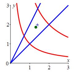
Thus the centroid for this region is \[\begin{aligned} \bar{x}&=\dfrac{A_x}{A}\approx\dfrac{1.37}{1.04}=1.31 \\ \bar{y}&=\dfrac{A_y}{A}\approx\dfrac{1.93}{1.04}=1.86 \end{aligned}\] The centroid is plotted in the region as a green circle.

Since the density \(\delta=\dfrac{xy}{2}\) increases with \(x\) and \(y\),
we expect the center of mass to be to the right and up from the centroid
which it is.
The center of mass is plotted in the region as a blue star.
The centroid is plotted in the region as a green circle.
Find the average density of the diamond region if the density is \(\delta=\dfrac{xy}{2}\).
There are two formulas for the average density, but they are equal: \[ \delta_\text{ave}=\dfrac{1}{A}\iint_R \delta\,dA =\dfrac{M}{A} \] since the integral of the density is the mass.
\(\displaystyle \delta_\text{ave}=\dfrac{5}{4}\)
The average density is simply the total mass divided by the area of the region, both of which we have already calculated: \[ \delta_\text{ave}=\dfrac{M}{A} =\dfrac{15\ln2}{8}\dfrac{2}{3\ln2} =\dfrac{5}{4} \]
Heading
Placeholder text: Lorem ipsum Lorem ipsum Lorem ipsum Lorem ipsum Lorem ipsum Lorem ipsum Lorem ipsum Lorem ipsum Lorem ipsum Lorem ipsum Lorem ipsum Lorem ipsum Lorem ipsum Lorem ipsum Lorem ipsum Lorem ipsum Lorem ipsum Lorem ipsum Lorem ipsum Lorem ipsum Lorem ipsum Lorem ipsum Lorem ipsum Lorem ipsum Lorem ipsum